4D lift of the tilings by the Smith et al. aperiodic monotile
Text written by Arnaud Chéritat
Work by Arnaud Chéritat and Nan Ma
Initial idea by Nan Ma
Contributions by Pieter Mostert
Introduction, motivation
In the articles An aperiodic monotile (March 2023) and A chiral aperiodic monitile (May 2023), David Smith, Joseph Samuel Myers, Craig S. Kaplan and Chaim Goodman-Strauss, hereafter designated as “the original authors”, discovered the first example of aperiodic monotile and chiral aperiodic monotile.
 |  | |
| Example of March tiling with the article's choice of wintery colors | Example of May tiling with spring hues |
The images were obtained via the web apps provided by the authors and linked from their dedicated web page for the March paper and similar page for the May paper.
A striking feature is that these monotiles belong to a one-parameter family of shapes, inducing in the case of the March paper a family of tilings that are combinatorially equivalent but such that transformations sending one to the other are necessarily geometrically elaborate.
The original authors also provided the following animation:
Animation downloaded from here.
I was finding it extremely mysterious. Especially, the dark blue tiles, which are approximately, but not exactly, centered on a trianglular lattice, seem to move slighlty off their position while they deform. The segments composing their boundaries rotate while they shrink/grow. The authors gave several hints of how to obtain those tilings but not a complete description of the algorithm and choices producing the animation.
Tile(a,b)
There are two important things to note:
1—When tiling a whole plane with the hat and its reflections, one necessarily has to put vertices on vertices and the segment colors must match. This is in fact true as soon as a > 0, b > 0 and a ≠ b.
On the other hand, with Tile(a,a) one can put red along green (more on this later).
2— Orientation of the boundary of Tile(a,b) as you wish. The sides come in parallel pairs with the same length and opposite orientation. (Since there is a set of 4 parallel red segments, the paring is not unique; it does not matter at this level.)
This has the consequence that in any tiling with the hat and its reflection, one can change the lengths of the red edges and the green edges to take respectively lengths a and b, with a ≥ 0 and b ≥ 0 chosen in advance: by point 2 each thusly modified tile boundary will close on itself (as the applet already showed); by point 1, any adjacent tile can be modified and placed so that the edges match on their common boundary. Actually the deformation of the tile is known in advance but the appropriate translation is only determined if a neighbouring tile's position has been determined.

1. Place deformed cyan tile as you wish. 2. This determines deformed yellow tile's position.
We can then start from one tile, positioned at will, and progressively position adjacent tiles, but it is sort of a leap of faith to believe that everything necessarily will fit together nicely without overlap or holes.

How it could go wrong.
It actually works and can be proved by decomposing the chain into elementary loops around vertices, a bit in the spirit of homology (or homotopy) theory. I will skip the details here.
Each vertex in a tiling moves relative to each other in a linear way with the parameters a,b. The relation is simple to work out for a single tile. However, considering the vertices of a complete tiling, there will be infinitely many different linear maps involved, in an intricate way.
The May tiling (spectres tiling) is initially performed with Tile(1,1).
The same deformations scheme can also be applied to this tiling.
However, this time, the deformed tiling displays two tiles: Tile(a,b) and Tile(b,a).
This is due to the fact that, now, some tiles sharing an edge are rotated by an odd multiple of 30 degrees with respect to each other.
But there was a third observation to make concerning the Tile(a,b) family:
3— The red vectors point in directions that are multiples of 60 degrees. The green vectors in directions that are odd multiple of 30°.
As a consequence, coming back to the two tiles, a red edge has to be glued to a green edge. This is not compatible with the deformation process, as illustrated below.

Choose any tile and use it as a reference. Call odd every tile whose orientation is an odd multiple of 30° degrees with respect to the reference tile. Call even the other ones. It is convenient to flip the red and green colouring of every edge of every odd tile, so that matching edges keep the same color and edges of a given color all have the same length. Since in every spectre tilings, there is a majority of even or odd tiles, we usually choose the reference tile among the majority so that odd tiles are the rare ones.
With that, it is possible to deform a whole tiling and the authors produced the following animation as a result, where the odd tiles are in white. (Their green vectors are my red vectors and their purple ones are my green...)
Animation downloaded from here.
The 4D lift
The outline of all tiles Tile(a,b) for various a and b can be seen as the projection of a single 4D path by the maps
defined by
The path is the concatenation of 14 segments in 4D of length 1, each of vector (x,y,0,0) or (0,0,x,y), as shown on the picture below.

There are 6 possible red vectors and 6 possible green vectors, leading to a total of 12 possible vector lifts. The 14 vectors ai cover all these possibilities. If the lower left vertex of Tile(1,1) is mapped to O = (0, 0, 0, 0) then vector a1 = (1, 0) is lifted to the vector
It is nice to be able to lift one tile, but Nan Ma understood that you can actually lift a whole tile arrangement. First, for any other tile rotated by 60 degrees and then possibly reflected along the horizontal axis, one can define a lift in the same way, and this amounts to take the lift of the initial tile and apply the rotation/reflection simultaneously to the two pairs of coordinates of each vertex. Then, two tiles adjacent along an edge have the same edge color and hence this edge lifts to the same vector for the two tiles. By a similar argument as the one I did not explain when I was commenting deformed tiles positioning above, this leads to a coherent lift of all vertices, coherent in the sense that for any edge of the tiling, the difference of the two lifted vertices coincides with the lift of the edge vector: the only condition is that the tiled area is simply connected. This condition is for instance satisfied for a tiling of the whole plane.
With this, he could produce this kind of videos.
The code for generating them is publicly available on this link. What is shown is the image of a static 4D object under a varying projection to ℝ3. Note that up to now I only described how to lift the outline of the tiles in a tiling, not the inside. There are several way to do this and the one above is one of them, more on this later. A finite patch of tiles has been lifted, their interiors filled and then this 4D surface has been projected to ℝ3 and then to the screen as follows: the two coordinates parallel to the screen are given by the map Lcos(t),sin(t) where t is a time parameter; the third coordinate has been chosen to be given by (x,y,x',y') ↦ −sin(t)×(x+y)+cos(t)×(x'+y'). The 3D engine (POV-Ray), a ray-tracer, then rendered material shine, shadows, etc. Denoting c=cos(t) and s=sin(t) the projection matrix is thus
| c | 0 | s | 0 |
| 0 | c | 0 | s |
| −s | −s | c | c |
This can adapt to the May tiling: when you lift an odd tile, do not forget to swap green and red vectors and that red goes to the first two coordinates and green goes to the last two coordinates.
Then you get the following video (more complete there)
I programmed an applet with which you can play with the animation and rotate the object in 3D.
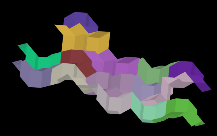
Click on the picture to access the applet page.
Again, what I particularly like with Nan Ma's approach is that, instead of having to think of a complicated articulated object with extensible rods, we just have to consider one static object, which we observe under different projections. On the downside, this object sits in 4D.
Observations
There are plenty of projections from 4D to 2D, so we can play with varying them. Also, the ways to fill-in the outlines are far from being unique, and we may also explore and maybe fill-in other outlines and vertices. I will report here some observations we made varying those projections, working with the tile outlines only.