4D lift of the tilings by the Smith et al. aperiodic monotile

Asymptotic plane

The first observation is that the lift stays at bounded distance from a plane that can be deduced from a substitution rule that the original authors indicated in their articles, and that both the March and the May tilings must obey. In the case of the March tiling, the substitution scheme is illustrated below by the original authors.

Copy of Figure 2.11 page 18 of the March preprint.

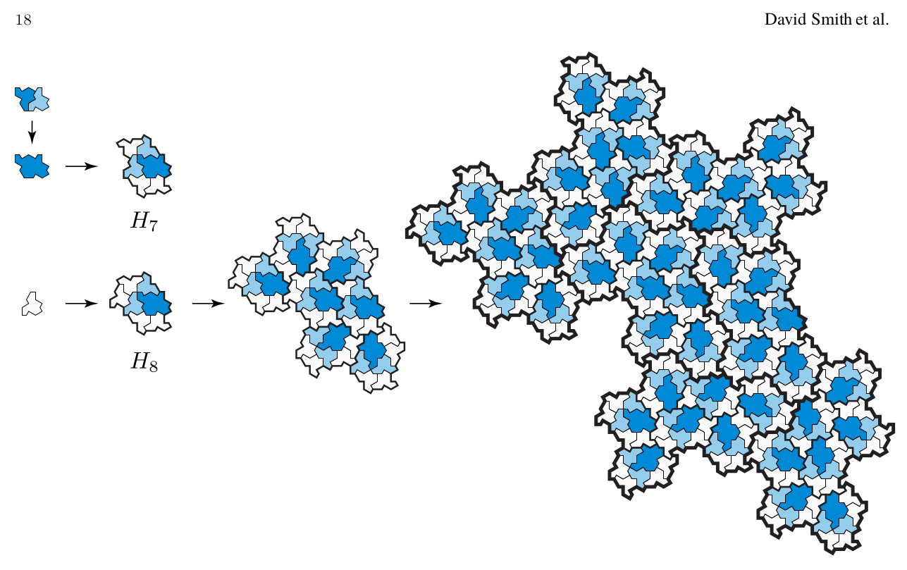
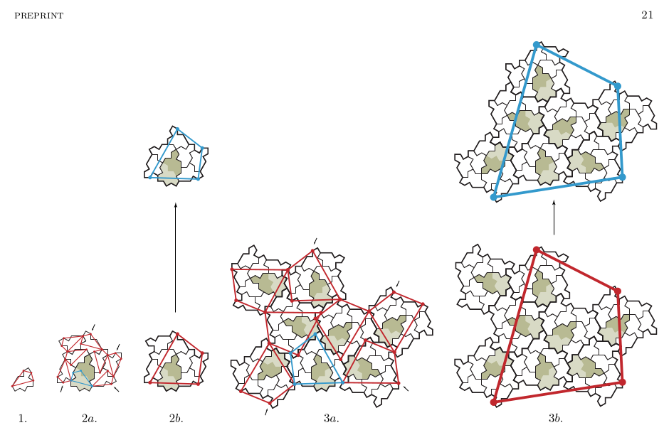
And in the case of the May article the figure is as below, with some added key points that turn out to be very convenient.

Copy of Figure A.1 page 21 of the May preprint.

The first figure did not indicate key points but Nan Ma was able to adapt to it the marking of the second figure. This is illustrated on the applet below, I will explain how it works.

The first thing to note is that, unlike most traditional substitution tilings like the Penrose tiling (or rather some modifications of it), this is not strictly an inflate-and-cut procedure. An integer called level will go from 0 to infinity. At each level, they define two clusters A and B of tiles. The definition is recursive: each level is an arrangement of clusters of the previous level. At the first level the clusters are quite simple: in A the odd tiles are amalgamated with a precise neighbourhing tile. Cluster B is just made of single even tiles. Each cluster also comes with 4 marked points on their boundaries. The level n+1 clusters A_n+1 and B_n+1 are obtained by arranging one A_n cluster and a certain number of B_n clusters by turning them by multiples of 60° and making some marked points match according to the map given by the illustrations.

It is far from obvious at all that the boundaries of the clusters will match but the original authors prove that their tiling* obeys the substitution rule, and this implies that the rule always works if started from a single tile or amalgamated tile.
*: Of course you must know that at least one tiling exists. For the May tiling, they use marked hexagons systems, that follow closely the substitution above. They obtained tilings by other means in the March paper, using another substitution system on what they call supertiles. Hexagons can be seen as a way to add markings on the tile boundaries and allow to prove directly that the substitution works. As a trade-off, the description is elaborate.

Below we analyse the consequences. In the following figure, note that one marked point is outside one of the clusters. It does not matter because it will not be used when we glue one copy of this cluster to 6 or 7 copies of the other cluster. Note also that the two quadrilaterals are identical for the two clusters.

Key points for the March tiling. For a change we took Tile(1,2), which is not exactly the hat (the latter being Tile(1,√3)).

Of particular interest are the vectors a, b, c, d between the marked points. Note that we have a+b+c+d = 0 but also d = ρ×c. These vectors can also be considered as complex numbers by identifying ℝ² and ℂ. Because of the relations above, they can be charaterized by, say, the pair (a,c). One has d=ρc and b = −a−(1+ρ)c, where ρ = exp(i 2π/6). By the figure above, one easily deduces the new values a', b', c', d' from those of a,b,c,d. Incidentally, one discovers that way (I won't include the computations here) that the arrangement of 7 quadrialterals closes up if and only if c and d are related by d=ρc.

We find that \[ \begin{bmatrix} a' \\ c' \end{bmatrix} = P \times \begin{bmatrix} a \\ c \end{bmatrix}\] with \[ P = \begin{bmatrix} 1+\rho & 2\rho^2 \\ -\rho & 1+\rho^{-1} \end{bmatrix} \] with j = ρ². The characteristic polynomial of the 2×2 complex matrix P is X²−3X+1, its eigenvalues are thus (3+√5)/2 and its inverse. The system is conjugated to the simpler matrix [[1,1],[1,2]] by using variables (c,e) with e = (a+ρc)/ρ², i.e. a=ρ²e−ρc.

One fun observation is that if the quadrilateral is isoceles (symmetric w.r.t. a line through two vertices) then its image is. This is the case of the quadrilateral of the turtle Tile(√3,1) for instance.

The substitution rule translates to a rule for the 4D lift of the tiles and clusters. The lifted versions of these vectors have two complex coordinates. They satisfy exactly the same relations a+b+c+d = 0 and d = ρc as above. And the expression of a', and c' in terms of a and c is the same, coordinate by coordinate, i.e. we have a block-diagonal matrix expression: \[ \begin{bmatrix} a'_{\mathrm{red}} \\ c'_{\mathrm{red}} \\ a'_{\mathrm{green}} \\ c'_{\mathrm{green}} \end{bmatrix} = \left[\begin{array}{c|c} P & 0 \\ \hline 0 & P \end{array}\right] \times \begin{bmatrix} a_{\mathrm{red}} \\ c_{\mathrm{red}} \\ a_{\mathrm{green}} \\ c_{\mathrm{green}} \end{bmatrix}\] From the fact that P has only one eigenvalue of modulus > 1 and every other (that means the other) has modulus < 1, it is standard to deduce from this that the substitution procedure yields only tilings whose lift are at bounded distance from some asymptotic one complex dimensional vector subspace of ℂ², whose asymptotic direction can be derived from the initial shape of the quadrilateral associated to the initial cluster B₀. We find that this direction is given by (z_red, z_green) ∈ ℂ² satisfying z_green = s × z_red with a slope \[s = \frac{\sqrt{3}-i\sqrt{5}}{4}.\] We call this the asymptotic plane though it is not an asymptote (the distance does not tend to 0), and if we allow it not to pass through 0, any plane parallel to it has the same property.

It makes sense to try and project to the asymptotic plane. This requires to choose a direction parallel to which it is done. That direction is given by a two dimensional vector subspace of ℝ⁴. If we endow ℝ⁴ with its canonical scalar product, one choice is the orthogonal of the projection plane. It is a one complex dimensional vector subspace of ℂ² too. (Actually for the canonical scalar product, the orthogonal of any ℂ-vector subspace of is a ℂ-vector subspace of ℂ², I leave this as an exercise.) The projection looks like this:

4D lift of March tiling orthogonally projected to asymptotic plane. Even tiles coloured according to their 6 possible orientations. Odd tiles coloured white independently of orientation.

Note: complex projections to ℂ of the 4D lift depend on two complex parameter, and if we consider them up to a similarity, they depend only on the quotient of these two parameters. The deformations of the tiling by the original authors correspond to the choice of a real quotient. It was already pointed-out by ZenoRogue on Mathstodon that one could take complex values of the parameters a,b in Tile(a,b). They made a nice animation.

The same analysis can be performed for the May tiling, for which we still have a+b+c+d=0 and d=ρc and we get a different induction relation: because the substitution rule induces an orientation reversal, the new vectors a', b', c' and d' satisfy c' = ρd' (instead of d' = ρc'). Taking two iterations of the transformation takes us back to the usual relation and we have \[ \begin{bmatrix} a'' \\ c'' \end{bmatrix} = Q \times \begin{bmatrix} a \\ c \end{bmatrix}\] (the matrix Q has the form \(\overline{P} P\) for some matrix P with coefficients in ℤ[ρ]). The matrix Q has characteristic polynomial X²-4X+1. We find that the asymptotic plane now has slope \[s = (\sqrt{15}-1)\frac{\sqrt{5}-3i}{14}.\] The orthogonal projection looks like this.

4D lift of May tiling orthogonally projected to asymptotic plane. Even tiles coloured according to their 6 possible orientations. Odd tiles coloured gray independently of orientation.

Instead of projecting to the asymptotic plane we may also want to project parallel to it. There is only one way up to similarity (contrarily to the projection to the asymptotic plane, which required to choose a complementary direction). I will call this here the defect projection because it is a way to measure the deviation of the vertices from the asymptotic plane. Before showing the pictures let me compare the projections of one tile parallel vs orthogonal to the asymptotic plane, and March vs May.

Comparison of different projections. The fill-in is purely decorative, because we only lifted and reprojected the outlines of the tiles, not their interiors. Reference points and anti-clockwise orientation has been put on the top row, and the corresponding orientation is indicated on the other two rows. The two yellow projections on the second row are very resemblant but different.

Note: The asymptotic planes of the March and the may tilings have a different slope. These planes make an "angle" close to 9.9°, which is rather small. The yellow tiles, which are, up to translation, the same subset of 4D space in both tilings, are somewhat parallel to either plane, which is coherent with the fact that their projections are very close: the cosine of 9.9° is very close to 1. However, computation shows that the red segments have an angle near 43° and the green ones near 47° with the March asymptotic plane, and for the May one the angles are close to 37.5° and 52.5°, so I don't know for sure.

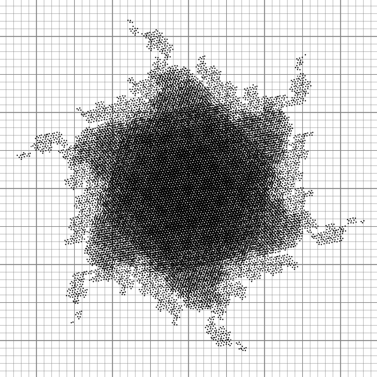
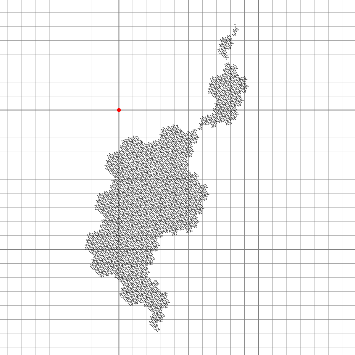
Let us show the projections of all vertices of a big patch, parallel to the asymptotic plane.

March tiling. Defect projections of all vertices of a big circular patch (17077 tiles, approximately 110,000 vertices). Scale: each thick line separated by 1. Projection: \( (z_1,z_2) \mapsto -\overline{s}z_1+z_2\) where s is the aforementioned March slope.

March tiling. Defect projections of all vertices of index 1 (tip of the head of the spectre) of only the tiles that are even and with a fixed orientation among the 6 possible (16,920 tiles). This is zoomed-in w.r.t. the previous picture. The origin is marked with a red dot.

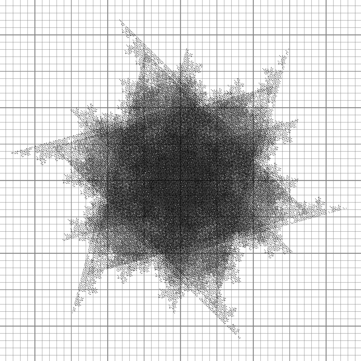
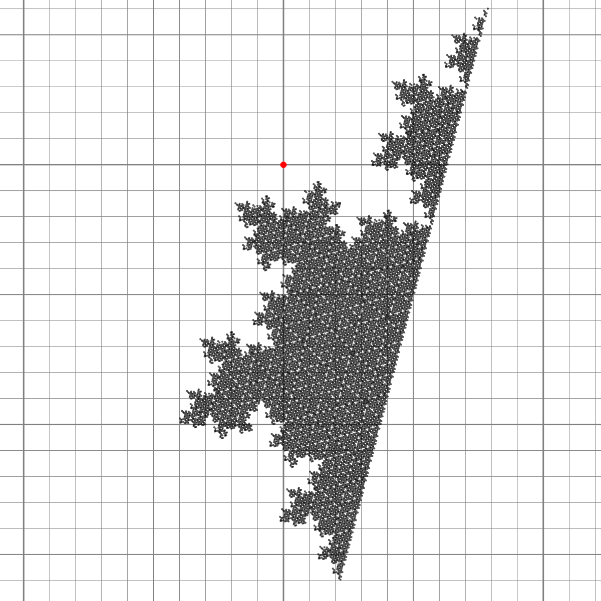
For other vertices and tile orientation we just get copies of the last pictures, translated if we fix the even tile orientation, rotated if we rotate it (the angle is the same), scaled down if we choose odd tiles with a given ortientation. At the limit, things get black and seem to cover bounded areas. This has to be bounded if we believe the previous claims made about the lift staying within bounded distance of the asymptotic plane.

Note for those who know this stuff: The second picture is reminiscent of a Rauzy type fractal and it hints at the fact that have a cut-and-project method with selection cylinder having a partially fractal boundary. I suppose there are standardized method to prove that but I will not try. It may be already proved in Dynamics and topology of the hat family of tilings, arXiv:2305.05639v2 by Michael Baake, Franz Gähler, and Lorenzo Sadun (they use a chomological language which I have not learned). And maybe elsewhere too.

May tiling. Defect projections of all vertices of a circular patch of 5848 tiles, (approximately 40,000 vertices) along the asymptotic plane to ℂ.

May tiling. Defect projections of all vertices of index 1 of only the tiles that are even and with a fixed orientation among the 6 possible (6861 tiles) along the asymptotic plane to ℂ.